Deriving the Rocket Equation from First Principles
The Tsiolkovsky Rocket Equation (hereafter referred to simply as “the rocket equation”) models the ultimate velocity of a rocket given its mass, the mass of fuel, and the velocity of the exhaust. While it may seem at first to be a straightforward relationship, the fundamental problem of rocketry is that a rocket must lift its own fuel. Say you want your 1000 kg rocket to accelerate to 1000 km/h, and you find that 200 kg of fuel has enough oomph to get 1000 kg up to that speed. So you fuel up your rocket, which now weighs 1200 kg, meaning it’s too heavy to get up to speed. So you have to add more fuel to lift the weight of the fuel. And again, and again and again…
The rocket equation prevents us from going through this iterative approach by giving an analytic solution to the problem. Risking accusations of spoilers, the rocket equation may be given as
in which
- is the total mass of the system (the rocket and the propellant)
- is the exhaust/propellant mass (this is used later)
- is the final mass of the rocket (all propellant has been used)
- is the exhaust velocity
- is the total change in ship’s velocity
Where does this equation come from? I was familiar with it as a tool, but I had always had it handed down from on high without explanation. So, I decided to give it a shot myself, under the following constraints and assumptions:
- I will only assume the law of conservation of momentum
- I will not research other derivations beforehand
- The universe consists only of this rocket and its fuel. I.e. there are no external forces to consider.
- Exhaust velocity is measured relative to the body of the rocket.
- The rocket starts from rest.
Initial Analysis
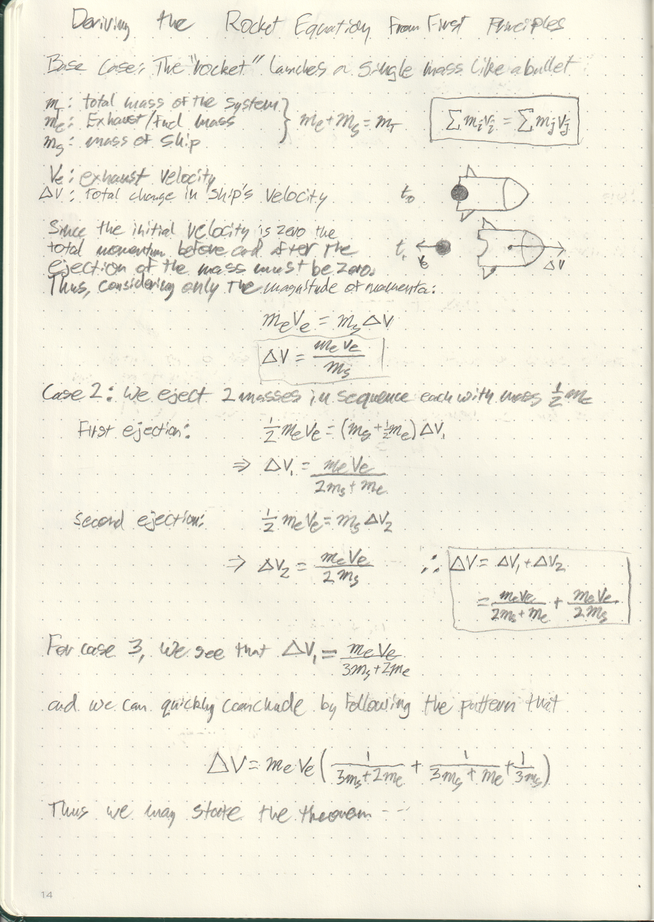
We begin by considering a “rocket” that propels itself by launching a single large mass in the opposite direction of its travel. This rocket is essentially a cannon, using a cannonball as propellant. We can then consider a rocket that fires two successive cannonballs, each with half the mass of the cannonball in the first design. Then we may consider a 3-shot design, a 4-shot, etc.
Since the rocket starts from rest, and we are only allowed the law of conservation of momentum, we may write
That is, the vector sum of all initial momenta at time must be zero and identical to the sum of all final momenta at time .
Case 1: A Single Propellant Ejection
The ejected propellant will have momentum that must be equal in magnitude to the momentum of the rocket . As we wish to solve for the final velocity of the rocket, we find
Case 2: Two sequential ejections
The first firing is calculated just as in the previous case, though we mustn’t forget that rocket still has extra mass from the remaining fuel.
The second and final ejection occurs while the rocket is already in motion. We simply add to the result of the second ejection.
Therefore
Case 3
Following the same procedure, we can see that and we can quickly conclude that the pattern extends to
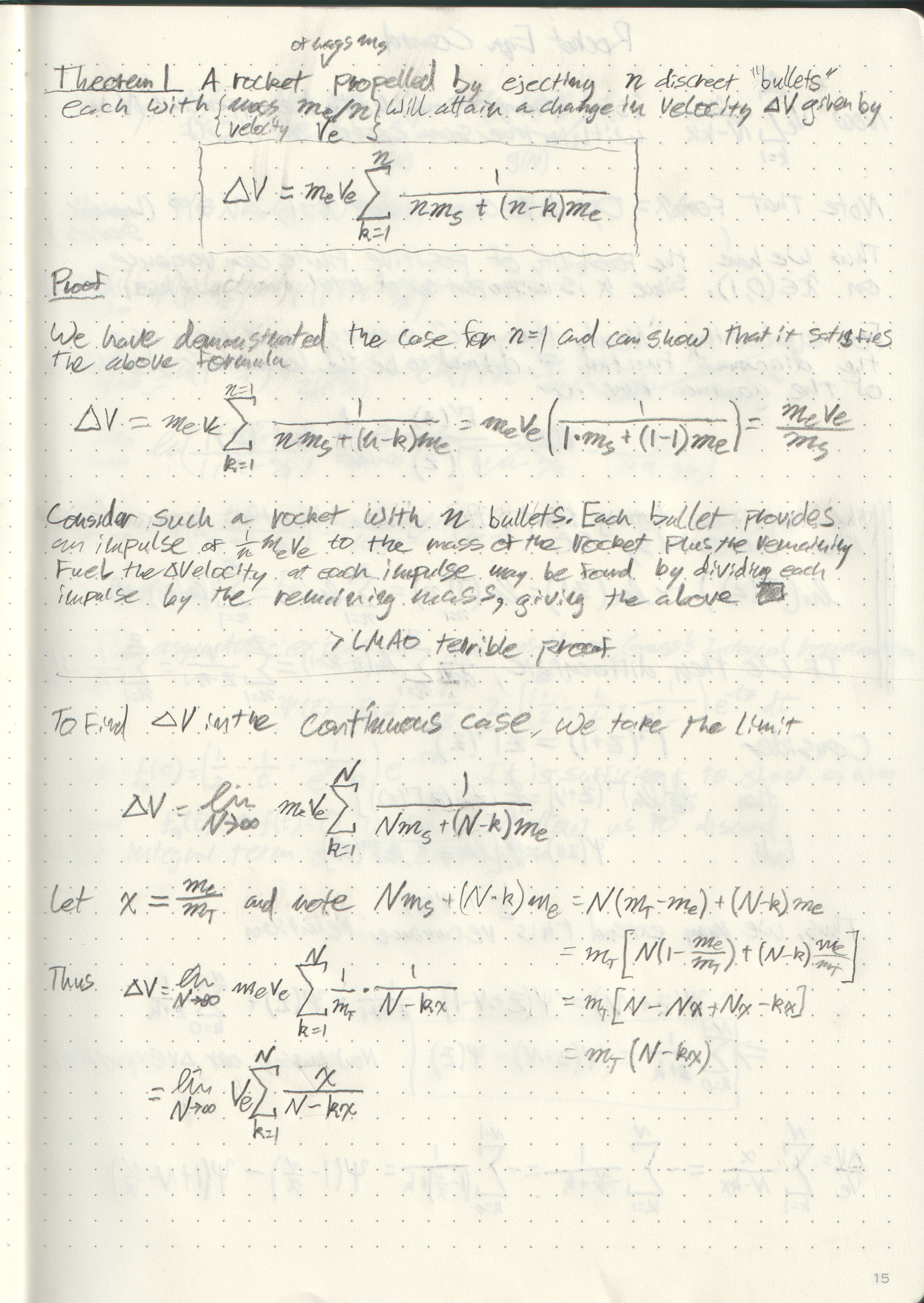
Theorem
A rocket of mass propelled by ejecting discreet “bullets” of mass at velocity will attain a total change in velocity given by
Having derived this series formula, we now wish to find a closed-form analytic solution.
From Discrete to Continuous
We can imagine as we increase the number of fuel ejections that the process goes from a series of distinct firings to a continuous stream of mass being ejected from the rocket. Indeed this is physically true: as the number of projectiles increases the share of mass for each decreases until the projectiles are individual atoms. Thus, we must take the limit as to correctly model an actual rocket.
We can modify the equation slightly by letting represent the proportion of total mass taken up by the fuel (note that this implies ). We can then use this substitution to rewrite the denominator
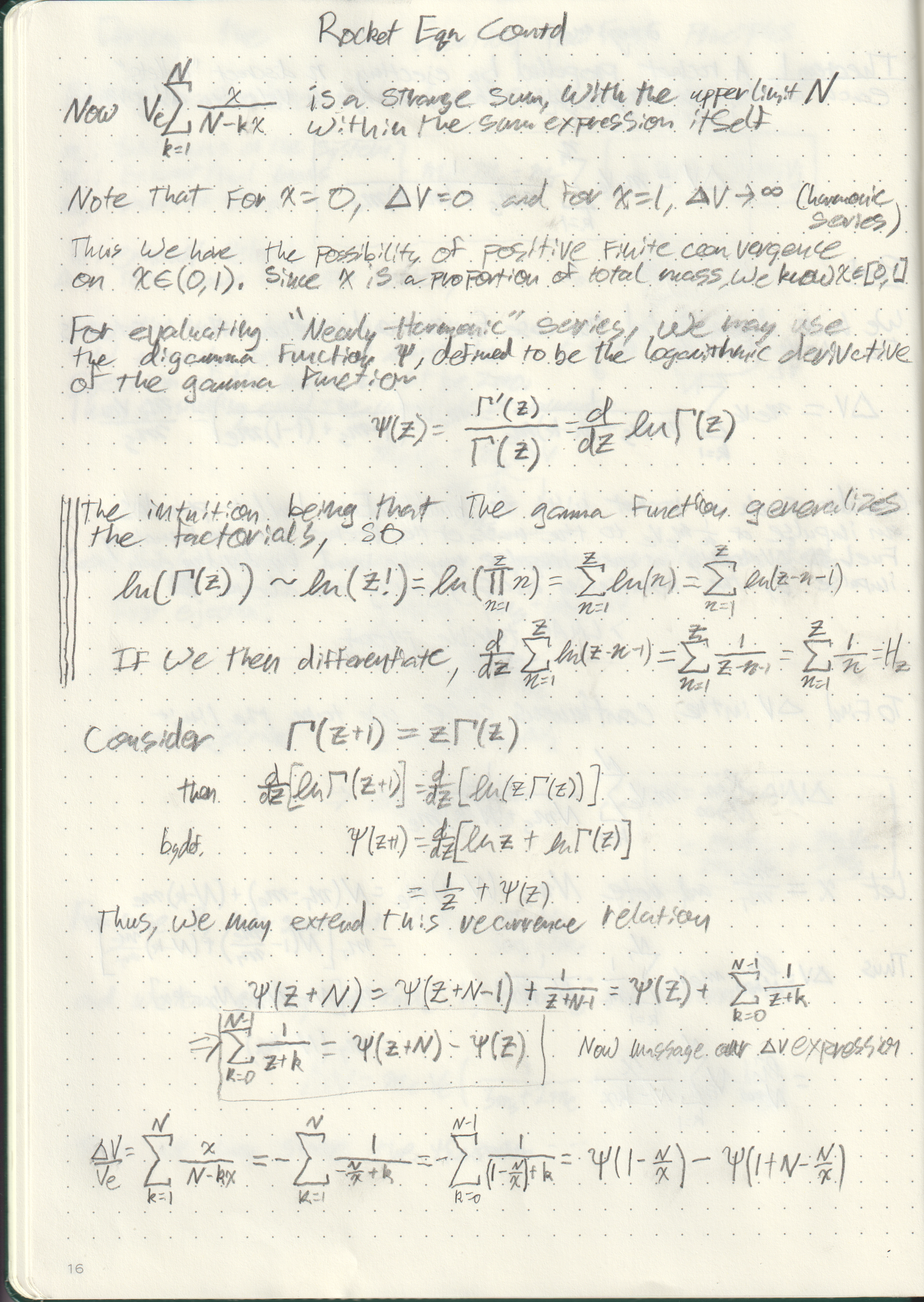
Though this expression is greatly simplified, we must contend with the unusual fact that the upper limit of the sum appears in the summation itself1. We expect the sum to converge for some values of since for , it is clear that and for , the sum becomes identical to the harmonic series and diverges. Thus it is likely that there is some positive finite value that is attained on the interval . This by no means proves convergence, but merely gives evidence for the possibility as well as motivation to continue our analysis.
To evaluate such a “nearly-harmonic” series we may use the digamma function, , defined as the logarithmic derivative of the gamma function
The intuition for the usefulness of the digamma function is that the gamma function generalizes the factorial, and the log of a product (like a factorial) becomes a sum.
Then by differentiating the above result, we have
Where is the harmonic number. The actual value of for some natural number is , supporting our intuition that the digamma function will be useful for computing a “nearly-harmonic” sum.
Theorem
Generalized recurrence relation for the digamma function
Proof: In order to use the digamma function to evaluate our sum, consider the defining recurrence relation of the gamma function . Taking the logarithmic derivative, we arrive at a recurrence relation for the digamma function
Now suppose that . Then for we have
We may now use this result to evaluate our rocket summation .
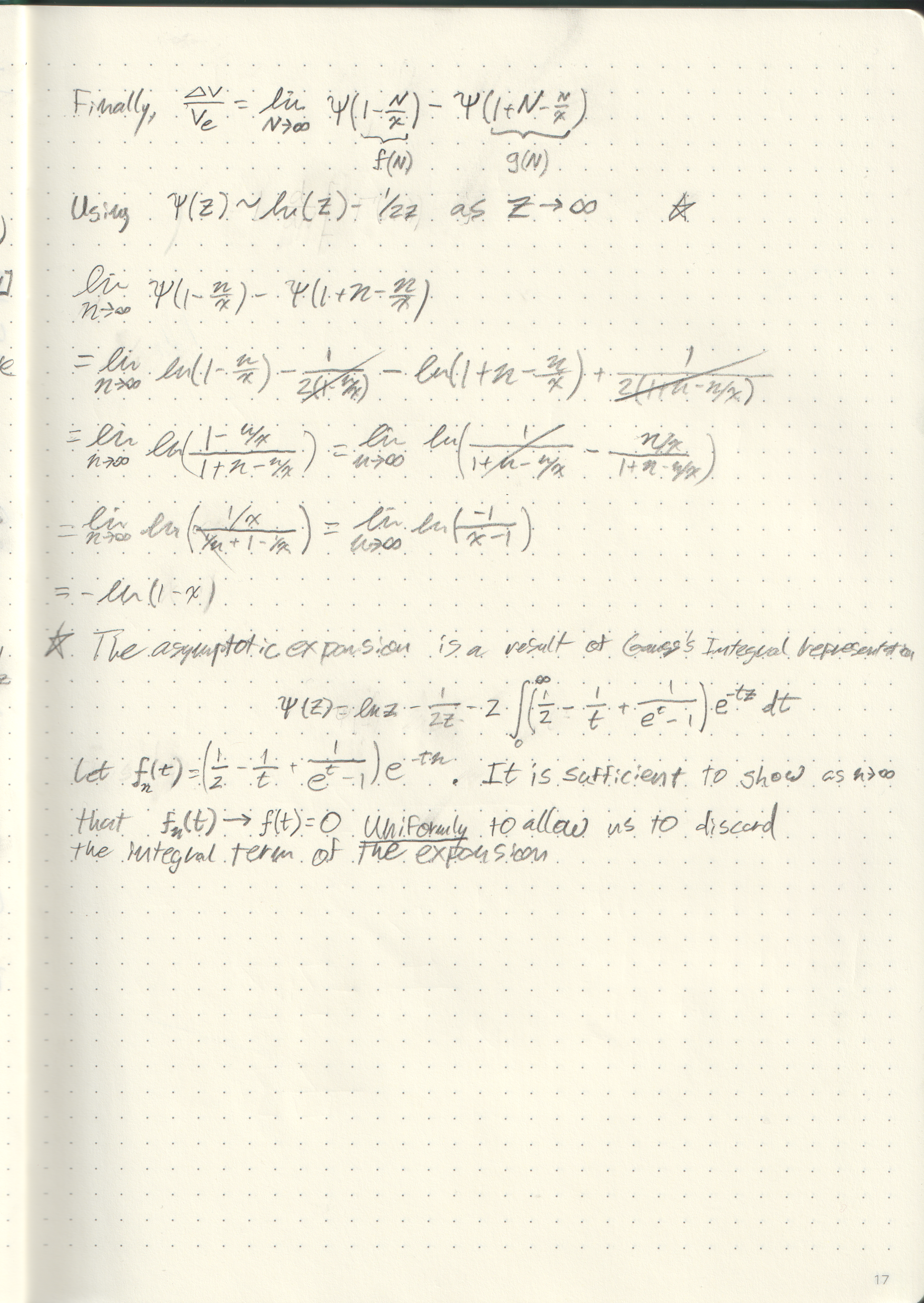
Now we are ready to take the limit as using the fact that as .
Thus the rocket equation is . After checking my work against the accepted form of the equation (which can be seen in the introduction), I saw that mass ratio used by most authors was . We can easily reframe our equation to match this form:
And we apply our last beautiful logarithm property to arrive precisely at our goal.
Closing thoughts
Other derivations of the rocket equation are certainly more elegant as they can take advantage of other physical laws. However, this nearly brute-force approach turned out to be deeply enlightening - I never would have expected the gamma function to come into play, for instance. Furthermore, I had never before had a chance to explore the digamma function. Without solving this problem, I doubt I would have had a chance to learn about it.
Solve hard problems in the wrong way. You’ll always learn something.
Scans of Relevant pages from my Notebook
-
At this point, most people would transform the sum into a Riemann integral to account for that term. It is the author’s opinion, however, that most people are cowards and quitters and integration is cheating. ↩︎